
Bean munging and Excel Wrangling
Messy Excel Files
So, as I discussed last time, the first big hurdle in starting to explore the domestic dry bean market data was overcoming the terror of working with a bunch of really messy, really gnarly excel files.
The main one looks like this: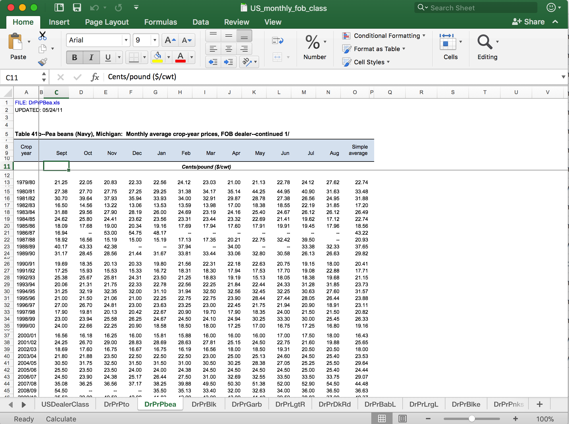
Lots of problems, right? The data are in multiple sheets in a single workbook, they’re not uniform, etc. It’s an R-user’s nightmare, but the reality is that data often look like this. So let’s get to work.
A brief point - here is the type of data we can expect from this workbook:
- year
- month
- day
- class (type of bean or variety)
- price
Step 1. Reading in the data
First things first, let’s load up some useful packages
library(tidyverse) ## Warning: package 'dplyr' was built under R version 3.5.1library(rJava)
library(readxl)
library(XLConnect)We’ll use the handy functions in readxl and XLConnect to read in the the excel sheets and then use tidyverse to do a bunch of stuff to them to clean them up.
All files can be found at my github repo for this project.
Download the appropriate files to your local working directory - and you’re ready to go.
Let’s read in the data with readxl’s loadWorkbook function (if you were better at making the RCurl package work than I am, you could pull it directly from my GitHub too):
#Loading Workbooks
dealer_price = loadWorkbook(file =
                      "/Users/KeatonWilson/Documents/Projects/beans2/data/Weekly_Dealer_price.xls")
#Remember your directory will be different

#Turning workbook into a list
dealer_price_list = readWorksheet(dealer_price, sheet = getSheets(dealer_price))

#Lots of errors with this, but don't worry.

#Looks good...lots of NAs, but there is data in there.
head(dealer_price_list[[1]], n = 20)
## Contents..Weekly.Dry.Bean.Prices..by.Class..and.Annual.Summary Col2
## 1 Source: USDA, Agricultural Marketing Service, Bean Market News <NA>
## 2 Last Updated: <NA>
## 3 <NA> <NA>
## 4 <NA> <NA>
## 5 Table 42--U.S. dry bean f.ob. dealer prices, 1981 <NA>
## 6 <NA> <NA>
## 7 Month Day
## 8 <NA> <NA>
## 9 <NA> <NA>
## 10 <NA>
## 11 <NA> <NA>
## 12 1 6
## 13 1 13
## 14 1 20
## 15 1 27
## 16 2 3
## 17 2 10
## 18 2 18
## 19 2 24
## 20 3 3
## Col3 Col4 Col5 Col6 Col7 Col8 Col9
## 1 <NA> <NA> <NA> <NA> <NA> <NA> <NA>
## 2 June 23, 1989 <NA> <NA> <NA> <NA> <NA> <NA>
## 3 <NA> <NA> <NA> <NA> <NA> <NA> <NA>
## 4 <NA> <NA> <NA> <NA> <NA> <NA> <NA>
## 5 <NA> <NA> <NA> <NA> <NA> <NA> <NA>
## 6 <NA> <NA> <NA> <NA> <NA> <NA> <NA>
## 7 Pinto Great Pink Small Navy Baby Large
## 8 <NA> Northern <NA> Red <NA> Lima Lima
## 9 <NA> <NA> <NA> <NA> <NA> <NA> <NA>
## 10 <NA> <NA> <NA> <NA> <NA> Dollars per Cwt <NA>
## 11 <NA> <NA> <NA> <NA> <NA> <NA> <NA>
## 12 32.00 31.75 31.75 36.25 27.25 27.75 38.50
## 13 32.75 32.25 31.50 36.50 29.25 34.00 38.00
## 14 35.50 33.25 34.00 36.50 30.00 36.00 37.50
## 15 35.25 33.75 33.88 35.75 30.50 38.50 37.50
## 16 35.25 34.25 34.50 36.00 30.75 39.50 38.00
## 17 34.75 34.25 34.50 36.50 31.25 39.50 39.50
## 18 35.00 35.50 34.50 36.75 31.75 40.50 40.50
## 19 35.00 35.50 34.50 36.75 31.75 41.50 40.50
## 20 34.25 35.25 34.25 36.25 32.88 44.50 40.50
## Col10 Col11 Col12 Col13 Col14
## 1 <NA> <NA> <NA> <NA> <NA>
## 2 <NA> <NA> <NA> <NA> <NA>
## 3 <NA> <NA> <NA> <NA> <NA>
## 4 <NA> <NA> <NA> <NA> <NA>
## 5 <NA> <NA> <NA> <NA> <NA>
## 6 <NA> <NA> <NA> <NA> <NA>
## 7 Blackeye Small Kidney Garbanzo <NA>
## 8 <NA> White <NA> <NA> <NA>
## 9 <NA> <NA> <NA> <NA> <NA>
## 10 <NA> <NA> <NA> <NA> <NA>
## 11 <NA> <NA> <NA> <NA> <NA>
## 12 26.75 33.25 31.50 37.00 <NA>
## 13 27.25 33.25 32.00 37.00 <NA>
## 14 28.50 33.50 32.75 37.00 <NA>
## 15 30.50 33.50 34.00 37.00 <NA>
## 16 31.00 33.50 34.25 37.50 <NA>
## 17 31.50 34.00 34.25 37.50 <NA>
## 18 31.25 34.25 34.50 37.50 <NA>
## 19 31.75 34.75 34.50 40.00 <NA>
## 20 32.75 34.75 34.25 41.00 <NA>Great! Now we have a list of the data from each year (where each item in the list is a dataframe of market data for different types of beans for each year).
If we look through all the dataframes in our list - there is a bunch of junk at the top of each one we need to get rid of. Let’s use the handy {r} lapply function for this.
#Bunch of garbage on the top of every data frame - need to iterate through the list and delete the first 11 rows
dealer_price_list = lapply(dealer_price_list, function(x) x[-c(1:11),])
head(dealer_price_list[[1]], n = 20)
## Contents..Weekly.Dry.Bean.Prices..by.Class..and.Annual.Summary Col2
## 12 1 6
## 13 1 13
## 14 1 20
## 15 1 27
## 16 2 3
## 17 2 10
## 18 2 18
## 19 2 24
## 20 3 3
## 21 3 10
## 22 3 17
## 23 3 24
## 24 3 31
## 25 4 7
## 26 4 14
## 27 4 21
## 28 4 28
## 29 5 5
## 30 5 12
## 31 5 19
## Col3 Col4 Col5 Col6 Col7 Col8 Col9 Col10 Col11 Col12 Col13 Col14
## 12 32.00 31.75 31.75 36.25 27.25 27.75 38.50 26.75 33.25 31.50 37.00 <NA>
## 13 32.75 32.25 31.50 36.50 29.25 34.00 38.00 27.25 33.25 32.00 37.00 <NA>
## 14 35.50 33.25 34.00 36.50 30.00 36.00 37.50 28.50 33.50 32.75 37.00 <NA>
## 15 35.25 33.75 33.88 35.75 30.50 38.50 37.50 30.50 33.50 34.00 37.00 <NA>
## 16 35.25 34.25 34.50 36.00 30.75 39.50 38.00 31.00 33.50 34.25 37.50 <NA>
## 17 34.75 34.25 34.50 36.50 31.25 39.50 39.50 31.50 34.00 34.25 37.50 <NA>
## 18 35.00 35.50 34.50 36.75 31.75 40.50 40.50 31.25 34.25 34.50 37.50 <NA>
## 19 35.00 35.50 34.50 36.75 31.75 41.50 40.50 31.75 34.75 34.50 40.00 <NA>
## 20 34.25 35.25 34.25 36.25 32.88 44.50 40.50 32.75 34.75 34.25 41.00 <NA>
## 21 34.25 35.50 34.25 36.12 33.00 49.50 39.75 33.50 35.50 34.25 41.00 <NA>
## 22 34.25 35.75 34.25 36.75 34.50 50.50 39.50 33.50 36.75 34.25 41.00 <NA>
## 23 34.50 36.00 35.50 36.00 34.75 50.50 39.50 33.50 37.50 34.25 41.50 <NA>
## 24 34.50 37.00 35.50 36.25 34.75 51.75 39.00 33.25 37.75 34.25 41.50 <NA>
## 25 34.88 38.00 36.25 35.75 34.50 52.00 39.00 33.25 38.00 34.25 41.00 <NA>
## 26 36.25 38.25 36.25 36.00 34.75 51.75 39.25 33.25 38.00 34.25 42.00 <NA>
## 27 36.25 38.25 36.50 36.00 34.75 51.75 39.00 33.25 38.00 34.25 43.50 <NA>
## 28 36.25 38.50 36.50 36.00 36.25 51.75 38.50 33.00 38.50 34.00 44.00 <NA>
## 29 37.00 38.50 36.75 36.00 40.50 51.50 38.50 32.75 42.50 34.00 44.00 <NA>
## 30 38.75 38.75 37.50 36.00 44.50 51.50 38.50 32.75 52.25 34.25 44.50 <NA>
## 31 43.50 39.25 38.50 37.50 46.25 51.50 38.50 32.75 52.50 35.00 44.50 <NA>Ok, now it gets gnarly.
Here is the problem - not all data frames have the same variables, and it looks like variable names are hidden somewhere down in each dataframe.
I ended up going through each data frame manually - obviously this doesn’t scale super well - and is laborious, but I couldn’t come up with a clever way to automate this, but here is an example of the type of code I used:
#1981
glimpse(dealer_price_list[[1]])
## Observations: 80
## Variables: 14
## $ Contents..Weekly.Dry.Bean.Prices..by.Class..and.Annual.Summary <chr> ...
## $ Col2 <chr> ...
## $ Col3 <chr> ...
## $ Col4 <chr> ...
## $ Col5 <chr> ...
## $ Col6 <chr> ...
## $ Col7 <chr> ...
## $ Col8 <chr> ...
## $ Col9 <chr> ...
## $ Col10 <chr> ...
## $ Col11 <chr> ...
## $ Col12 <chr> ...
## $ Col13 <chr> ...
## $ Col14 <chr> ...dealer_price_list[[1]]## Contents..Weekly.Dry.Bean.Prices..by.Class..and.Annual.Summary Col2
## 12 1 6
## 13 1 13
## 14 1 20
## 15 1 27
## 16 2 3
## 17 2 10
## 18 2 18
## 19 2 24
## 20 3 3
## 21 3 10
## 22 3 17
## 23 3 24
## 24 3 31
## 25 4 7
## 26 4 14
## 27 4 21
## 28 4 28
## 29 5 5
## 30 5 12
## 31 5 19
## 32 5 27
## 33 6 2
## 34 6 9
## 35 6 16
## 36 6 23
## 37 6 30
## 38 7 7
## 39 7 14
## 40 7 21
## 41 7 28
## 42 8 4
## 43 8 11
## 44 8 18
## 45 8 25
## 46 9 1
## 47 9 9
## 48 9 15
## 49 9 22
## 50 9 29
## 51 10 6
## 52 10 14
## 53 10 20
## 54 10 27
## 55 11 3
## 56 11 10
## 57 11 17
## 58 11 24
## 59 12 1
## 60 12 8
## 61 12 16
## 62 12 22
## 63 12 29
## 64 <NA>
## 65 = =
## 66 <NA> <NA>
## 67 <NA> <NA>
## 68 <NA> <NA>
## 69 Monthly Average Dry Bean Prices, $/cwt 1981 <NA>
## 70 - -
## 71 Month <NA>
## 72 - -
## 73 <NA> <NA>
## 74 <NA> <NA>
## 75 Jan <NA>
## 76 Feb <NA>
## 77 Mar <NA>
## 78 Apr <NA>
## 79 May <NA>
## 80 Jun <NA>
## 81 Jul <NA>
## 82 Aug <NA>
## 83 Sep <NA>
## 84 Oct <NA>
## 85 Nov <NA>
## 86 Dec <NA>
## 87 <NA> <NA>
## 88 Ave * <NA>
## 89 = =
## 90 * = Calendar year simple average. <NA>
## 91 N/A = Not available. <NA>
## Col3 Col4 Col5 Col6 Col7 Col8 Col9
## 12 32.00 31.75 31.75 36.25 27.25 27.75 38.50
## 13 32.75 32.25 31.50 36.50 29.25 34.00 38.00
## 14 35.50 33.25 34.00 36.50 30.00 36.00 37.50
## 15 35.25 33.75 33.88 35.75 30.50 38.50 37.50
## 16 35.25 34.25 34.50 36.00 30.75 39.50 38.00
## 17 34.75 34.25 34.50 36.50 31.25 39.50 39.50
## 18 35.00 35.50 34.50 36.75 31.75 40.50 40.50
## 19 35.00 35.50 34.50 36.75 31.75 41.50 40.50
## 20 34.25 35.25 34.25 36.25 32.88 44.50 40.50
## 21 34.25 35.50 34.25 36.12 33.00 49.50 39.75
## 22 34.25 35.75 34.25 36.75 34.50 50.50 39.50
## 23 34.50 36.00 35.50 36.00 34.75 50.50 39.50
## 24 34.50 37.00 35.50 36.25 34.75 51.75 39.00
## 25 34.88 38.00 36.25 35.75 34.50 52.00 39.00
## 26 36.25 38.25 36.25 36.00 34.75 51.75 39.25
## 27 36.25 38.25 36.50 36.00 34.75 51.75 39.00
## 28 36.25 38.50 36.50 36.00 36.25 51.75 38.50
## 29 37.00 38.50 36.75 36.00 40.50 51.50 38.50
## 30 38.75 38.75 37.50 36.00 44.50 51.50 38.50
## 31 43.50 39.25 38.50 37.50 46.25 51.50 38.50
## 32 45.50 39.25 39.00 37.00 45.75 52.00 38.50
## 33 45.00 40.00 39.50 37.50 45.75 51.50 38.37
## 34 45.25 40.25 39.50 37.50 45.50 51.50 38.50
## 35 44.50 40.25 69.00 36.50 45.50 51.50 38.50
## 36 44.50 40.00 38.50 37.00 44.50 51.00 38.50
## 37 43.25 40.00 36.00 36.00 43.75 51.50 38.50
## 38 42.50 40.00 35.50 35.50 43.50 51.00 39.00
## 39 41.00 39.25 <NA> <NA> 42.75 50.25 38.50
## 40 36.50 37.50 <NA> <NA> 38.50 48.50 39.00
## 41 <NA> <NA> <NA> <NA> 36.00 47.50 39.00
## 42 32.25 35.50 <NA> <NA> 33.00 46.00 49.50
## 43 31.25 35.25 30.00 32.00 33.00 44.00 39.50
## 44 29.50 34.75 <NA> 29.00 31.00 43.00 39.50
## 45 28.25 31.00 <NA> <NA> 29.50 37.00 39.50
## 46 25.25 30.50 <NA> <NA> 28.50 33.00 39.50
## 47 23.50 28.88 <NA> <NA> 29.00 <NA> <NA>
## 48 23.75 28.75 24.00 25.00 29.00 31.00 40.50
## 49 22.75 27.75 23.00 26.50 31.00 30.50 40.50
## 50 22.00 27.50 23.75 26.75 34.50 30.50 40.50
## 51 22.25 31.00 23.00 26.50 42.00 30.50 40.50
## 52 22.38 32.00 22.75 26.50 39.50 31.00 41.25
## 53 22.25 31.00 23.00 26.25 39.50 30.50 41.00
## 54 22.00 30.75 22.75 26.00 38.75 30.50 41.00
## 55 21.75 30.75 22.75 26.00 39.50 30.50 41.00
## 56 21.75 30.75 22.25 25.25 38.00 30.50 41.00
## 57 21.75 30.50 22.75 25.00 38.00 30.25 40.75
## 58 21.50 30.25 22.75 25.00 36.25 30.25 40.25
## 59 20.88 30.25 <NA> 23.00 36.50 30.00 40.00
## 60 20.25 30.00 <NA> 22.00 36.25 29.75 39.75
## 61 18.75 30.25 <NA> 22.00 35.50 29.00 39.25
## 62 18.25 28.75 <NA> 22.00 36.00 29.00 39.25
## 63 17.62 28.25 <NA> 22.00 35.50 28.25 38.25
## 64 <NA> <NA> <NA> <NA> <NA> <NA> <NA>
## 65 = = = = = = =
## 66 <NA> <NA> <NA> <NA> <NA> <NA> <NA>
## 67 <NA> <NA> <NA> <NA> <NA> <NA>
## 68 <NA> <NA> <NA> <NA> <NA> <NA> <NA>
## 69 <NA> <NA> <NA> <NA> <NA> <NA> <NA>
## 70 - - - - - - -
## 71 Pinto Grt.Nort. Pink S_Red Navy B_Lima L_lima
## 72 - - - - - - -
## 73 <NA> <NA> <NA> <NA> <NA> $/cwt <NA>
## 74 <NA> <NA> <NA> <NA> <NA> <NA> <NA>
## 75 33.88 32.75 32.78 36.25 29.25 34.06 37.88
## 76 35.00 34.88 34.50 36.50 31.38 40.25 39.63
## 77 34.35 35.90 34.75 36.27 33.98 49.35 39.65
## 78 35.91 38.25 36.38 35.94 35.06 51.81 38.94
## 79 41.19 38.94 37.94 36.63 44.25 51.63 38.50
## 80 44.50 40.10 44.50 36.90 45.00 51.40 38.47
## 81 40.00 38.92 35.50 35.50 41.58 49.92 38.83
## 82 30.31 34.13 30.00 30.50 31.63 42.50 42.00
## 83 23.45 28.68 23.58 26.08 30.40 31.25 40.25
## 84 22.22 31.19 22.88 26.31 39.94 30.63 40.94
## 85 21.69 30.56 22.63 25.31 37.94 30.38 40.75
## 86 19.15 29.50 -- 22.20 35.95 29.20 39.30
## 87 <NA> <NA> <NA> <NA> <NA> <NA> <NA>
## 88 $31.80 $34.48 $32.31 $32.03 $36.36 $41.03 $39.59
## 89 = = = = = = =
## 90 <NA> <NA> <NA> <NA> <NA> <NA> <NA>
## 91 <NA> <NA> <NA> <NA> <NA> <NA> <NA>
## Col10 Col11 Col12 Col13 Col14
## 12 26.75 33.25 31.50 37.00 <NA>
## 13 27.25 33.25 32.00 37.00 <NA>
## 14 28.50 33.50 32.75 37.00 <NA>
## 15 30.50 33.50 34.00 37.00 <NA>
## 16 31.00 33.50 34.25 37.50 <NA>
## 17 31.50 34.00 34.25 37.50 <NA>
## 18 31.25 34.25 34.50 37.50 <NA>
## 19 31.75 34.75 34.50 40.00 <NA>
## 20 32.75 34.75 34.25 41.00 <NA>
## 21 33.50 35.50 34.25 41.00 <NA>
## 22 33.50 36.75 34.25 41.00 <NA>
## 23 33.50 37.50 34.25 41.50 <NA>
## 24 33.25 37.75 34.25 41.50 <NA>
## 25 33.25 38.00 34.25 41.00 <NA>
## 26 33.25 38.00 34.25 42.00 <NA>
## 27 33.25 38.00 34.25 43.50 <NA>
## 28 33.00 38.50 34.00 44.00 <NA>
## 29 32.75 42.50 34.00 44.00 <NA>
## 30 32.75 52.25 34.25 44.50 <NA>
## 31 32.75 52.50 35.00 44.50 <NA>
## 32 32.75 52.50 35.50 44.50 <NA>
## 33 33.50 52.50 38.00 44.50 <NA>
## 34 35.50 52.50 39.00 44.50 <NA>
## 35 37.50 50.50 39.50 44.50 <NA>
## 36 40.62 50.50 39.50 44.50 <NA>
## 37 40.50 50.00 39.50 44.50 <NA>
## 38 39.50 49.00 39.50 46.00 <NA>
## 39 39.00 49.50 38.50 45.00 <NA>
## 40 37.75 <NA> 38.25 44.75 <NA>
## 41 37.50 47.00 38.00 44.50 <NA>
## 42 36.25 <NA> 37.50 44.50 <NA>
## 43 34.50 <NA> 36.00 46.00 <NA>
## 44 32.50 <NA> 34.00 46.00 <NA>
## 45 32.00 <NA> 32.50 46.00 <NA>
## 46 31.50 <NA> 33.50 46.00 <NA>
## 47 <NA> <NA> <NA> <NA> <NA>
## 48 29.50 <NA> 31.25 46.00 <NA>
## 49 28.50 <NA> 30.25 46.00 <NA>
## 50 28.00 36.75 31.50 46.00 <NA>
## 51 28.25 44.50 32.50 46.00 <NA>
## 52 28.25 43.00 33.50 46.00 <NA>
## 53 28.25 42.75 32.50 47.50 <NA>
## 54 28.25 42.25 32.00 47.50 <NA>
## 55 28.50 42.25 31.50 48.00 <NA>
## 56 29.00 42.00 31.25 50.00 <NA>
## 57 29.50 41.75 32.00 50.00 <NA>
## 58 29.50 41.75 32.50 50.00 <NA>
## 59 29.75 41.75 32.50 50.00 <NA>
## 60 29.75 41.00 32.00 50.00 <NA>
## 61 29.75 39.50 32.00 50.00 <NA>
## 62 39.75 39.50 31.50 50.00 <NA>
## 63 39.75 39.50 31.50 50.00 <NA>
## 64 <NA> <NA> <NA> <NA> <NA>
## 65 = = = =
## 66 <NA> <NA> <NA> <NA> <NA>
## 67 <NA> <NA> <NA> <NA> <NA>
## 68 <NA> <NA> <NA> <NA> <NA>
## 69 <NA> <NA> <NA> <NA> <NA>
## 70 - - - - <NA>
## 71 Blackeye S_White Kidney Garbanzo <NA>
## 72 - - - - <NA>
## 73 <NA> <NA> <NA> <NA> <NA>
## 74 <NA> <NA> <NA> <NA> <NA>
## 75 28.25 33.38 32.56 37.00 <NA>
## 76 31.38 34.13 34.38 38.13 <NA>
## 77 33.30 36.45 34.25 41.20 <NA>
## 78 33.19 38.13 34.19 42.63 <NA>
## 79 32.75 49.94 34.69 44.38 <NA>
## 80 37.52 51.20 39.10 44.50 <NA>
## 81 38.75 49.25 38.75 45.25 <NA>
## 82 33.81 -- 35.00 45.63 <NA>
## 83 29.38 36.75 31.63 46.00 <NA>
## 84 28.25 43.13 32.63 46.75 <NA>
## 85 29.13 41.94 31.81 49.50 <NA>
## 86 33.75 40.25 31.90 50.00 <NA>
## 87 <NA> <NA> <NA> <NA> <NA>
## 88 $32.45 $41.32 $34.24 $44.25 <NA>
## 89 = = = = <NA>
## 90 <NA> <NA> <NA> <NA> <NA>
## 91 <NA> <NA> <NA> <NA> <NA>dealer_price_list[[1]] = dealer_price_list[[1]][-c(64:100),-14]
colnames(dealer_price_list[[1]]) = c("Month", "Day", "Pinto", "Grt_Northern", "Pink", "Sm_Red", "Navy", "B_Lima", "L_Lima", "Blackeye",
"Small_White", "Kidney", "Garbanzo")
glimpse(dealer_price_list[[1]])## Observations: 63
## Variables: 13
## $ Month <chr> "1", "1", "1", "1", "2", "2", "2", "2", "3", "3",...
## $ Day <chr> "6", "13", "20", "27", "3", "10", "18", "24", "3"...
## $ Pinto <chr> "32.00", "32.75", "35.50", "35.25", "35.25", "34....
## $ Grt_Northern <chr> "31.75", "32.25", "33.25", "33.75", "34.25", "34....
## $ Pink <chr> "31.75", "31.50", "34.00", "33.88", "34.50", "34....
## $ Sm_Red <chr> "36.25", "36.50", "36.50", "35.75", "36.00", "36....
## $ Navy <chr> "27.25", "29.25", "30.00", "30.50", "30.75", "31....
## $ B_Lima <chr> "27.75", "34.00", "36.00", "38.50", "39.50", "39....
## $ L_Lima <chr> "38.50", "38.00", "37.50", "37.50", "38.00", "39....
## $ Blackeye <chr> "26.75", "27.25", "28.50", "30.50", "31.00", "31....
## $ Small_White <chr> "33.25", "33.25", "33.50", "33.50", "33.50", "34....
## $ Kidney <chr> "31.50", "32.00", "32.75", "34.00", "34.25", "34....
## $ Garbanzo <chr> "37.00", "37.00", "37.00", "37.00", "37.50", "37....Look at how nice that looks! Now it’s time to iterate through all the dataframes. You may be thinking to yourself, “Hey, why don’t you do that with a loop, or with lapply?”. That’s a great idea… except that dataframes vary in their content. Manual brute-force it is.
Let’s skip ahead a bit - with a bit more munging and cleaning, we end up with a very nice long-format dataframe, that you can find here.
Or alternatively:
dealer_price_long = read_csv(file = "https://raw.githubusercontent.com/keatonwilson/beans/master/data/dealer_price_long.csv?token=AefUVKUxTssySEILhpmU2TOfE32UocJfks5bq6gMwA%3D%3D")## Parsed with column specification:
## cols(
## date = col_date(format = ""),
## Class = col_character(),
## Price = col_double()
## )dealer_price_long ## # A tibble: 23,984 x 3
## date Class Price
## <date> <chr> <dbl>
## 1 1981-01-06 Pinto 32
## 2 1981-01-13 Pinto 32.8
## 3 1981-01-20 Pinto 35.5
## 4 1981-01-27 Pinto 35.2
## 5 1981-02-03 Pinto 35.2
## 6 1981-02-10 Pinto 34.8
## 7 1981-02-18 Pinto 35
## 8 1981-02-24 Pinto 35
## 9 1981-03-03 Pinto 34.2
## 10 1981-03-10 Pinto 34.2
## # ... with 23,974 more rowsAlso note that this is in tibble format now. Thanks, Hadley. :)
Conclusions
This is a great start. We went from an awful Excel Workbook to a slim and trim tidy dataframe with ~24,000 entries of bean prices from 1981-2010 - this is going to be a big chunk of the data we end up splitting into training and test sets down the road for Machine Learning.
A small aside - there was a bunch of munging and cleaning involved between some of the steps above. If you’re interested in a deeper dive into what was entailed, check out the full source code - it’s pretty well annotated and can give you a nice look at things.
Cheers!

