
Bean Market Predictions using Machine Learning Algorithms
Goals
As I’ve discussed in earlier posts, the basic premise of this project was to use a nice (but messy) dataset from the USDA on domestic bean markets to explore a variety of different avenues of analysis, visualization and data exploration. One of the main goals of this project was to see if I could build some machine learning models that do a good job of predicting future prices of different classes of beans.
In past posts we’ve worked to import messy data from Excel files, and preprocessing data using the caret package to make sure it’s ready for running some building, testing and tuning some machine learning algorithms.
We’re going to start with the preprocessed data set outlined in my last post. Let’s give it a lookover to remind ourselves what’s in it (and load up our packages)
library(tidyverse)
library(caret)

glimpse(bean_ML_import_train)
## Observations: 6,101
## Variables: 13
## $ date <date> 1987-01-13, 1987-01-21, 1987-01-27, ...
## $ class <fct> Pinto, Pinto, Pinto, Pinto, Pinto, Pi...
## $ price <dbl> -1.454833, -1.501566, -1.517986, -1.5...
## $ whole_market_avg <dbl> -0.4745942, -0.5321818, -0.5238085, -...
## $ whole_market_sum <dbl> -0.7998774, -0.8469529, -0.8401081, -...
## $ class_market_share <dbl> -0.59721573, -0.60937574, -0.62198404...
## $ planted <dbl> 1.748686, 1.748686, 1.748686, 1.74868...
## $ harvested <dbl> 1.860342, 1.860342, 1.860342, 1.86034...
## $ yield <dbl> -0.5854438, -0.5854438, -0.5854438, -...
## $ production <dbl> 1.827526, 1.827526, 1.827526, 1.82752...
## $ month <fct> January, January, January, February, ...
## $ imports <dbl> 1.923680, 1.923680, 1.923680, 1.92368...
## $ future_monthly_avg_price <dbl> 20.23250, 20.23250, 20.23250, 18.5950...glimpse(bean_ML_import_test)## Observations: 1,524
## Variables: 13
## $ date <date> 1987-03-10, 1987-09-01, 1987-09-09, ...
## $ class <fct> Pinto, Pinto, Pinto, Pinto, Pinto, Pi...
## $ price <dbl> -1.6038740, -1.5255645, -1.5647192, -...
## $ whole_market_avg <dbl> -1.08451367, -1.48155901, -1.73468560...
## $ whole_market_sum <dbl> -1.656314940, -2.599220377, -1.829949...
## $ class_market_share <dbl> -0.3291083, 0.4656110, -0.1993913, 0....
## $ planted <dbl> 1.748686, 1.748686, 1.748686, 1.74868...
## $ harvested <dbl> 1.860342, 1.860342, 1.860342, 1.86034...
## $ yield <dbl> -0.5854438, -0.5854438, -0.5854438, -...
## $ production <dbl> 1.827526, 1.827526, 1.827526, 1.82752...
## $ month <fct> March, September, September, October,...
## $ imports <dbl> 1.923680, 1.865905, 1.923680, 1.86590...
## $ future_monthly_avg_price <dbl> 18.0300, 17.6520, 17.6520, 17.3450, 2...So these dataframes look great - remember that the values look a little wonky because we’ve centered and scaled them, and that the overall goal is to predict future monthly average price given everything else. We can also look at the dimensions of the data frames (6101 rows in our training set and 1524 rows in our test set) - these make sense too, based on our previous training and test splits.
Our basic ML pipeline is this:
Preprocess > Split > Model Building > Model Testing > Model Tuning
Let’s jump into some algorithms.
It’s worth talking a little bit about algorithm choice. In general, there are two big categories of predictive algorithms. First, there are those that predict classes (putting observations into categories based on other variables - think of things like tumor identification, identifying customers who might unsubscribe to a service (churn), or determining if a certain wine variety belongs in one cluster over another).
The second are algorithms that output continuous, numeric values given a set of input variables (things like average customer rating of a book, the price of cryptocurrencies or, in our case the price of a hundred-weight of beans). I’ll cover classifcation algorithms in another post, and will focus on a variety of continuous predictors here. A brief aside here - we’ll also be focusing exclusively on supervised learning - unsupervised learning typically adresses a differnt set of questions (taking unlabeled data and finding patterns or classifcations within the data set) - here, we have a different goal - generate good predictive models.
There are a bazillion different algorithms, which can be a bit daunting at first, but we’ll explore a few of the basics here:
1. Linear Regression
2. Classification and Regression Tree (CART)
3. Artificial Neural Net (ANN)
4. Random Forest
All of these algorithms have pros and cons. For example, linear regressions provide fairly interpretable mechanics (that is, we can see what the model is doing to extract what variables are the most important and how they’re interacting), whereas neural netss are great at predicting really complex phenomena, but are computationally expensive (you’ll see below that they can take a long time to run), and are black boxes (i.e. it’s hard for humans to interpret what’s happening inside them).
Linear Regression
Let’s start with the old standby of analysis - the linear regression. If you want a refresher on how this works, check out this. In its simplest form, regression models predict variability in one continuous variable based on another, generating a line that best predicts this relationship. This get’s a little more complicated when the model incorporates information on many different variables, and interactions between those variables, but… that’s not what this post is about.
In all of the examples, we’ll be implementing the caret package to run the models.
The first step is to setup an object that will allow us to control parameters across all the m
library(caret)

#setting seed for reproducibility:
set.seed(42)
fitControl = trainControl(method = "repeatedcv", number = 5, repeats = 5)
The trainControl function here lets us build this object. If you check out the help page for the function, you can see there are LOTS of arguments - you have a lot of control over what happens in your models. Here, we’re specifying that we’re going to use repeated cross validation (check out this), with 5 repeats and 5 folds (this is fairly robust, and we might have reduce it later on for the ANN). Because these are example models, I’m using a smaller number of repeats and folds, which can help us do quicker model assement before diving in deeper to tune models.
Now we can run our model:
A warning - this takes a while, mostly because we’re doing a lot of model comparisons. The train function is splitting the training data into 10 different training and test sets 10 different times, AND also using the grid argument in trainControl to modifying different model parameters of the linear regression to tune the model simulatenously.
#And just a standard linear model
lmfit1 = train(future_monthly_avg_price ~ ., data = bean_ML_import_train,
               method = "lm",
               trControl = fitControl)
Next, we can inspect our model, and also examine how well it did on in-sample data.
lmfit1## Linear Regression
##
## 6101 samples
## 12 predictor
##
## No pre-processing
## Resampling: Cross-Validated (5 fold, repeated 5 times)
## Summary of sample sizes: 4881, 4879, 4882, 4881, 4881, 4880, ...
## Resampling results:
##
## RMSE Rsquared MAE
## 5.365845 0.5593651 4.111581
##
## Tuning parameter 'intercept' was held constant at a value of TRUENot bad! You can see from the output that we have an RMSE (Root-Mean Squared Error) of 5.4, which means that on average, the model predicts bean price within $5.4 per hundred-weight, and an R-squared of 0.559 The model is only explaining around 56% of the variance in price. Remember, this is only an estimate on in-sample data using k-fold cross validation - the actual effectivness of the model might be different on test data.
Also, the MAE parapmeter stands for Mean Absolute Error, and is another parameter we can asseess our model’s fit with - also in the same units as the dependent variable (just like RMSE). A nice comparison of RMSE and MAE can be found here.
We could try and tune the model, and run it on out-of-sample test data, but let’s move on to some more models.
Classification and Regression Tree Models
CART stands for Classification and Regression Tree. These models are a type of decision tree model, an overview of which can be found here if you’re interested in the machinery under the hood.
cartfit1 = train(future_monthly_avg_price ~ ., data = bean_ML_import_train,
                 method = "rpart",
                 trControl = fitControl)
## Warning in nominalTrainWorkflow(x = x, y = y, wts = weights, info =
## trainInfo, : There were missing values in resampled performance measures.cartfit1## CART
##
## 6101 samples
## 12 predictor
##
## No pre-processing
## Resampling: Cross-Validated (5 fold, repeated 5 times)
## Summary of sample sizes: 4882, 4880, 4879, 4882, 4881, 4880, ...
## Resampling results across tuning parameters:
##
## cp RMSE Rsquared MAE
## 0.0433896 6.003610 0.4477434 4.657532
## 0.1162622 6.480589 0.3562770 5.035152
## 0.3085252 7.520604 0.2895985 5.969671
##
## RMSE was used to select the optimal model using the smallest value.
## The final value used for the model was cp = 0.0433896.So this model is worse than the old-fashioned linear regression! The best model here generates an RMSE of 6.00 and an R-squared of 0.45 - the model is predicting 45% of the variance in market prices 6 months ahead of time - not bad!
Let’s try running the model on our out-of-sample test set.
We use two functions to do this - first the predict function, which we feed our model and the test-data set. This will use the model to build some predictions of price 6 months ahead of time which we can then compare to the actual prices in thes test set.
We can do this comparison with the postResample function from caret, which compares the mean-squared error and R-squared for our predicted values and the actual values of the test set.
p_cartfit1 = predict(cartfit1, bean_ML_import_test)

postResample(pred = p_cartfit1, obs = bean_ML_import_test$future_monthly_avg_price)
## RMSE Rsquared MAE
## 6.0397584 0.4233428 4.7287406So, pretty close to the measures of model performance obtained with 5-fold cross validation, though a bit worse. Overall, we’re improving though.
We could go back and tune the CART model, by changing the tuneLength argument in the train function, but let’s do this on a later model - we’re starting to get to the good stuff!
Artificial Neural Net
Neural nets were designed to mimic how our brains and biological communication systems function. They’re made up of a collection of units or nodes and can transmit information to each other. Deep neural nets that allow information to travel all around the network are en vogue right now, but are computationally expensive - here, we’ll used a paired down version, again with the caret package.
nnfit2 = train(future_monthly_avg_price ~ ., data = bean_ML_import_train,
               method = "nnet",
               trControl = fitControl,
               maxit = 100,
               linout = 1,
               verbose = FALSE)
## Warning in nominalTrainWorkflow(x = x, y = y, wts = weights, info =
## trainInfo, : There were missing values in resampled performance measures.Here, we specify the linout argumnet as TRUE in the train function - this lets the function know that we’re interested in a linear output - otherwise a sigmoidal activation function is used, and all the predictions will be constrained between 0 and 1.
nnfit2## Neural Network
##
## 6101 samples
## 12 predictor
##
## No pre-processing
## Resampling: Cross-Validated (5 fold, repeated 5 times)
## Summary of sample sizes: 4880, 4880, 4881, 4881, 4882, 4880, ...
## Resampling results across tuning parameters:
##
## size decay RMSE Rsquared MAE
## 1 0e+00 8.080127 NaN 6.501369
## 1 1e-04 8.080127 NaN 6.501369
## 1 1e-01 7.881306 0.1241743 6.330698
## 3 0e+00 8.080127 NaN 6.501369
## 3 1e-04 8.080127 NaN 6.501369
## 3 1e-01 7.449453 0.4798837 5.950023
## 5 0e+00 8.080127 NaN 6.501369
## 5 1e-04 8.080127 NaN 6.501369
## 5 1e-01 7.255844 0.4153007 5.773972
##
## RMSE was used to select the optimal model using the smallest value.
## The final values used for the model were size = 5 and decay = 0.1.p_nnetfit2 = predict(nnfit2, bean_ML_import_test)
postResample(pred = p_nnetfit2, obs = bean_ML_import_test$future_monthly_avg_price)## RMSE Rsquared MAE
## 5.2056459 0.5697035 4.0592629Here, the best model in our tuning grid was one with an RMSE of $7.71/hundredweight of beans in in-sample data, which resulted in an RMSE of 7.9 on out-of-sample test data. Unfortunately, we can’t extract R^2s from these data (a finciky bit of the nnet function, which I can’t find an answer to!). Regardless, not much better than our linear regression. Let’s move on.
Random Forest
Random forests algorithms are a type of ensemble learning method - the idea is to construct a ton of different decision trees, and outputting the mean prediction of all of the individual trees. Here, we use the caret pacakge again, with the ranger function.
This is going to take a while if you run it yourself…
rffit1 =  train(future_monthly_avg_price ~ ., data = bean_ML_import_train,
                        method = "ranger",
                        trControl = fitControl)

rffit1
## Random Forest
##
## 6101 samples
## 12 predictor
##
## No pre-processing
## Resampling: Cross-Validated (5 fold, repeated 5 times)
## Summary of sample sizes: 4882, 4881, 4882, 4879, 4880, 4881, ...
## Resampling results across tuning parameters:
##
## mtry splitrule RMSE Rsquared MAE
## 2 variance 3.469872 0.8684889 2.7045488
## 2 extratrees 4.922189 0.7763186 3.9290863
## 16 variance 1.465102 0.9685482 0.8722360
## 16 extratrees 1.512769 0.9683322 0.9566884
## 30 variance 1.506020 0.9661231 0.8499988
## 30 extratrees 1.469716 0.9695850 0.9027341
##
## Tuning parameter 'min.node.size' was held constant at a value of 5
## RMSE was used to select the optimal model using the smallest value.
## The final values used for the model were mtry = 16, splitrule =
## variance and min.node.size = 5.Woooooooo man! Look at those scores! The best model has an R^2 of 0.97, and an RMSE of 1.515! This is by far the best model we’ve tested so far. It’s explaining 97% of the variance in future average monthly price!
Let’s see how it does on out-of-sample data.
p_rffit2 = predict(rffit1, bean_ML_import_test)

postResample(pred = p_rffit2, obs = bean_ML_import_test$future_monthly_avg_price)
## RMSE Rsquared MAE
## 1.2342623 0.9765519 0.7254784Fantastic - the model appears to have similar performance on the test data! Let’s see if we can tune the model a bit more to get a bit more predictive power.
rffit2 =  train(future_monthly_avg_price ~ ., data = bean_ML_import_train,
                        method = "ranger",
                        trControl = fitControl,
                        tuneLength = 5)

rffit2
## Random Forest
##
## 6101 samples
## 12 predictor
##
## No pre-processing
## Resampling: Cross-Validated (5 fold, repeated 5 times)
## Summary of sample sizes: 4881, 4881, 4881, 4880, 4881, 4880, ...
## Resampling results across tuning parameters:
##
## mtry splitrule RMSE Rsquared MAE
## 2 variance 3.484480 0.8672428 2.7130311
## 2 extratrees 4.912424 0.7758483 3.9211817
## 9 variance 1.563117 0.9647930 0.9655579
## 9 extratrees 1.633444 0.9638930 1.0733833
## 16 variance 1.461370 0.9687225 0.8721647
## 16 extratrees 1.516951 0.9680933 0.9593576
## 23 variance 1.448004 0.9689824 0.8435539
## 23 extratrees 1.479318 0.9693886 0.9200007
## 30 variance 1.490552 0.9668369 0.8483187
## 30 extratrees 1.471178 0.9695186 0.9023834
##
## Tuning parameter 'min.node.size' was held constant at a value of 5
## RMSE was used to select the optimal model using the smallest value.
## The final values used for the model were mtry = 23, splitrule =
## variance and min.node.size = 5.This model took some time to run and tune, and we’ve improved the in-sample prediction slightly. Let’s test it out on the test data.
p_rffit3 = predict(rffit2, bean_ML_import_test)

postResample(pred = p_rffit3, obs = bean_ML_import_test$future_monthly_avg_price)
## RMSE Rsquared MAE
## 1.2236033 0.9767012 0.6869148This results in significant improvements - with better RMSE, Rsquared and MAE values compared to the un-tuned model.
Finally, let’s take a look at how to visualize how well our model does.
#binding the predictions onto the test set
bean_ML_import_test$pred = predict(rffit1, newdata = bean_ML_import_test)
#generating a plot of actual prices versus predicted future prices
ggplot(bean_ML_import_test, aes(x = pred, y = future_monthly_avg_price, color = class)) +
geom_point() +
theme_classic() +
geom_abline(slope = 1, intercept = 1) +
xlab("Predicted Future Price") +
ylab("Actual Future Price ")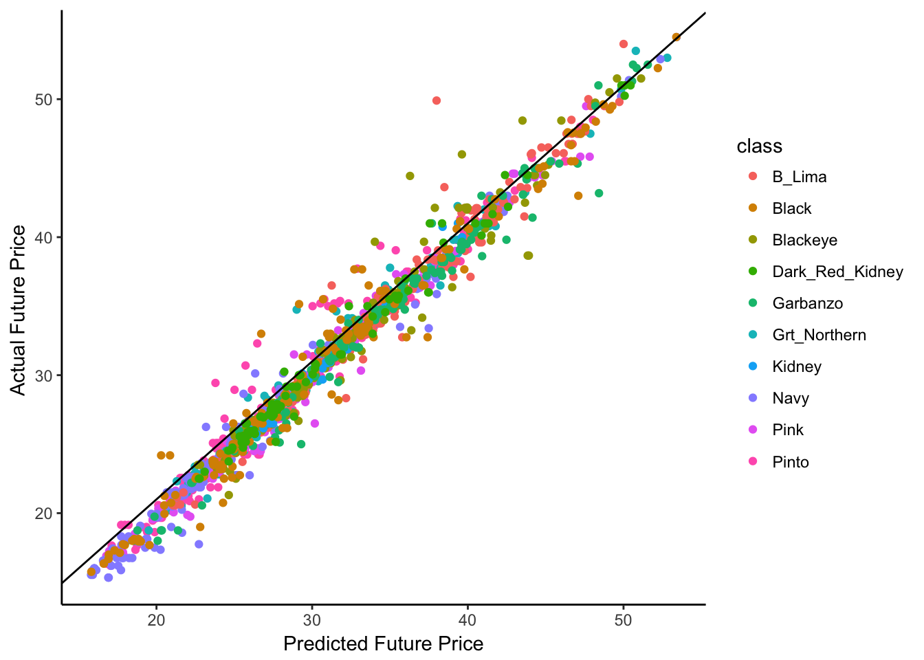 The black diagonal line represents the 1:1 line, dots on this line are when our model is doing a perfect job of predicting. Points above this line are scenarios where our model under-predicted price, and dots below are when the model over-predicted price. One interesting trend is that you can see that though most dots are really close to the line, many are just below, indicating that our model consistently slightly over-predicts price - something to keep in mind if this was going to be used for by investors.
#We can also plot this over time for each variety
bean_ML_import_test$date = as.Date(bean_ML_import_test$date)
bean_ML_import_test %>%
gather(key = valuetype, value = future_price, pred, future_monthly_avg_price) %>%
ggplot(aes(x = date, y = future_price, color = class, lty = factor(valuetype))) +
geom_path() +
theme_classic() +
facet_wrap( ~ class) +
ylab("Future Price ($)") +
xlab("Date") +
scale_linetype_discrete(name = "",
labels = c("Actual Future Price", "Predicted Future Price")) +
scale_color_discrete(name = "Variety")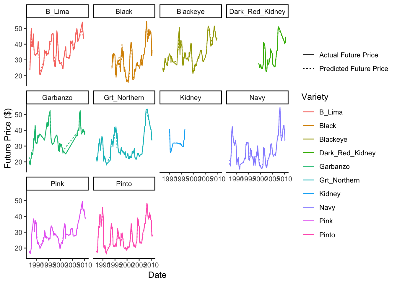 Overall this figure matches the first figure - our model is doing a great job over time at prediction.
Conclusions
Overall, this post outlines one of the main goals I was working towards on this project - to develop a machine learning model that does a good job of predicting future bean prices based on current information. The best model here does a pretty amazing job at this - predicting the average monthly price six months into the future within $1.20/hundredweight across all classes. You can imagine how useful this type of predictive model might be for individuals or businsses interested in speculating on the market.
In the next few posts, we’ll look at some other interesting data from this project - and I’ll introduce a basic investing/portfolio model I’ve built on the Machine Learning model outlined here to demonstrate how much money someone could make if they had used this model to trade beans during this period. Pretty interesting stuff!
Cheers!

