
Machine Learning Algorithm for Tucson Housing Prices
Introduction
The goal of this project has three main components: 1) to scrape a bunch of web data of house information in Tucson (prices, beds, baths, some other stuff), 2) to build a test a series of machine learning models that do a good job of accurately predicting the price a house will sell at and 3) taking this model and building a web interface that folks could use to plug in information on a house in Tucson and get an output.
I’m not going to cover the first part of the project because of the murkiness of web-scraping, but so we’ll start with part 2 here and hopefully get to part 3 in the upcoming weeks!
Loading and cleaning the data
First, we’ll need to load up some packages (there will be quite a few for this).
#Packages
library(skimr) #I like this better than glimpse
library(tidyverse) #The usual suspects
library(caret) #Machine Learning
library(recipes) #PreProcessing Recipes
library(lubridate) #We'll do some date stuff
library(rsample) #Sampling for ML
library(caretEnsemble) #Ensemble models
library(doParallel) #Parallel Processing to speed things up a bit
We’ll set up the parallel processing and set the seed.
#parallel
detectCores()
## [1] 4registerDoParallel(cores = 4)
#seed
set.seed(42)Now we’ll get into the nitty gritty of some data cleaning before we use the recipes package to pre-process the data.
#Reading in the data
housing_df = read_csv("/Users/KeatonWilson/Documents/Projects/Tucson_Housing_Machine_Learning/data/housing_df.csv") #I'm pulling this from my local directory - email me if you want to play with the data.
## Warning: Missing column names filled in: 'X1' [1]## Parsed with column specification:
## cols(
## X1 = col_integer(),
## address = col_character(),
## price = col_double(),
## dens = col_integer(),
## beds = col_integer(),
## baths = col_double(),
## zip = col_integer(),
## sqft = col_integer(),
## date_sold = col_date(format = ""),
## lat = col_double(),
## lon = col_double()
## )housing_df## # A tibble: 30,170 x 11
## X1 address price dens beds baths zip sqft date_sold lat
## <int> <chr> <dbl> <int> <int> <dbl> <int> <int> <date> <dbl>
## 1 1 878 Ha… 907660 811 NA NA 85624 1118 2018-01-17 31.5
## 2 2 Casita… 415000 272 NA NA 85624 1524 2018-01-17 31.5
## 3 3 10 Aco… 430000 229 NA 2 85624 1872 2017-01-31 31.5
## 4 4 33 Kim… 240000 93 NA 3 85624 2560 2016-12-14 31.5
## 5 5 6 Acor… 249000 186 3 1 85624 1337 2016-05-24 31.5
## 6 6 5920 E… 340000 136 4 3 85739 2490 2018-09-19 32.5
## 7 7 39779 … 418989 107 4 5 85739 3896 2018-06-14 32.5
## 8 8 6080 E… 310000 132 5 3 85739 2343 2018-03-05 32.5
## 9 9 12640 … 275000 147 2 2 85619 1870 2016-05-04 32.4
## 10 10 6234 N… 649000 305 2 2 85750 2121 2018-12-20 32.3
## # ... with 30,160 more rows, and 1 more variable: lon <dbl>#Doing a bit of cleaning after looking at the data
housing_df = housing_df %>%
select(-X1, -address) %>%
mutate(zip = as.factor(zip),
month = month(date_sold),
day = day(date_sold)) %>%
select(-date_sold)
#Take a look at the data using skim
skim(housing_df)## Skim summary statistics
## n obs: 30170
## n variables: 10
##
## ── Variable type:factor ─────────────────────────────────────────────────────────────────────────────────────────────────────
## variable missing complete n n_unique
## zip 0 30170 30170 45
## top_counts ordered
## 857: 3195, 857: 2713, 857: 2250, 857: 1541 FALSE
##
## ── Variable type:integer ────────────────────────────────────────────────────────────────────────────────────────────────────
## variable missing complete n mean sd p0 p25 p50 p75 p100
## beds 6288 23882 30170 3.16 0.91 2 3 3 4 22
## day 244 29926 30170 16.66 8.93 1 9 16 25 31
## dens 4431 25739 30170 121.84 51.77 1 92 119 147 986
## sqft 4263 25907 30170 1934.16 4443.84 1 1296 1636 2140 275000
## hist
## ▇▁▁▁▁▁▁▁
## ▃▆▆▇▅▅▅▇
## ▇▆▁▁▁▁▁▁
## ▇▁▁▁▁▁▁▁
##
## ── Variable type:numeric ────────────────────────────────────────────────────────────────────────────────────────────────────
## variable missing complete n mean sd p0 p25
## baths 4655 25515 30170 2.2 0.91 0.5 2
## lat 31 30139 30170 32.16 0.31 31.33 32.1
## lon 31 30139 30170 -111.04 0.51 -119.42 -111.13
## month 244 29926 30170 8.68 3.12 1 6
## price 0 30170 30170 2e+05 150552.48 1 98000
## p50 p75 p100 hist
## 2 2 37 ▇▁▁▁▁▁▁▁
## 32.2 32.32 41.6 ▇▁▁▁▁▁▁▁
## -111.01 -110.92 -73.09 ▁▇▁▁▁▁▁▁
## 10 11 12 ▁▁▂▁▂▃▂▇
## 170000 245000 992000 ▆▇▂▁▁▁▁▁#Looking at the distribution of prices to see if anything is wonky
ggplot(housing_df, aes(x = price)) +
geom_histogram()## `stat_bin()` using `bins = 30`. Pick better value with `binwidth`.
#Removing houses that cost very little (probably errors in price generation)
housing_df = housing_df %>%
  filter(price > 50000)

#removing dens at it has price built in
housing_df = housing_df %>%
  select(-dens)

#Removing entries with really wrong lats and lons
housing_df = housing_df %>%
  filter(lat < 33)
Great! Now we have a semi-clean data set that contains a lot of useful data to predict price with.
Specifically:
1. Price
2. Bedrooms
3. Bathrooms
4. Zip Code
5. Square feet
6. Date Sold
7. Latitude and Longitude
We need to split into training and test sets and also pre-process (transform, impute) before we start building algorithms.
#Split into train and test using some tools from the rsample package
train_test_split = initial_split(housing_df)
housing_train = training(train_test_split)
housing_test = testing(train_test_split)

#Check for missing
sum(is.na(housing_df))
## [1] 6989#A LOT of missing, but we can try and impute
tucson_rec = recipe(price ~ ., data = housing_train) %>%
#step_log(price, base = 10) %>%
step_bagimpute(all_numeric()) %>% #imputation
step_YeoJohnson(beds, baths, sqft, -lat, -lon) %>% #YeoJohnson Transformation
step_center(beds, baths, sqft, -lat, -lon) %>% #Centering
step_scale(beds, baths, sqft, -lat, -lon) %>% #Scaling
step_dummy(all_nominal()) %>% #One Hot Encoding
step_bs(lat, lon) #Splines
#Rational for step_bs - Makes sense to include splines above given the complex relationship between lat, lon and price.
housing_train %>%
filter(lat < 33) %>%
ggplot(aes(y = price, x = lat)) +
geom_point(alpha = 0.2) +
geom_smooth() +
theme_classic()## `geom_smooth()` using method = 'gam' and formula 'y ~ s(x, bs = "cs")'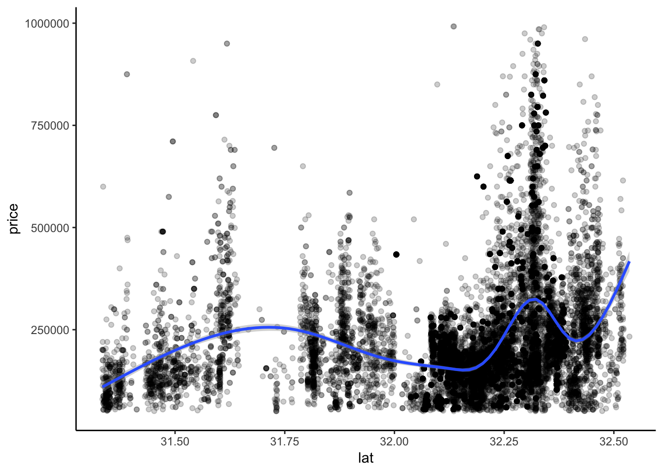
housing_train %>%
  filter(lat < 33) %>%
  ggplot(aes(y = price, x = lon)) +
  geom_point(alpha = 0.2) +
  geom_smooth() +
  theme_classic()
## `geom_smooth()` using method = 'gam' and formula 'y ~ s(x, bs = "cs")'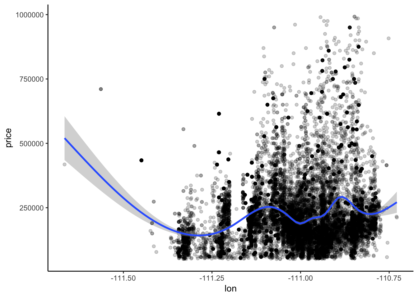
#Prepping the data
prepped_tucson = prep(tucson_rec, training = housing_train)

#Generating preprocessed training and test data
train_data = bake(prepped_tucson, new_data = housing_train)
test_data = bake(prepped_tucson, new_data = housing_test)
## Warning in bs(x = c(32.5148575, 32.4391429, 32.3137296, 32.312586,
## 32.308355, : some 'x' values beyond boundary knots may cause ill-
## conditioned bases## Warning in bs(x = c(-110.8679814, -110.7563179, -110.8415315,
## -110.846994, : some 'x' values beyond boundary knots may cause ill-
## conditioned basesSingle-Algorithm Testing and Tuning
Now the fun begins! We can start to build and test different algorithms to try and predict price. We’ll assess models using repeated cross-validation, and do a bit of automatic tuning along the way. Some of these models take a long time - the Random Forest and XGBoost in particular. I’ll be loading saved models (RDS objects) to save computational time and not re-build models I’ve already done, but I’ll also provide code on exactly how to work through each model.
Linear Regression
#Setting up the train control object telling caret we want to use repeated cross validation (3 folds with 3 repeats).

train_control = trainControl(method = "repeatedcv", number = 3, repeats = 3)
#Tune Length is longer here because linear models are fast - not wise to do this on a random forest.
lm_mod = train(price ~ ., data = train_data,
method = "lm", trControl = train_control, tuneLength = 10)#loading the RDS object to save time - this won't work for you.
lm_mod = readRDS("/Users/KeatonWilson/Documents/Projects/Tucson_Housing_Machine_Learning/output/lm_model.rds")
summary(lm_mod)##
## Call:
## lm(formula = .outcome ~ ., data = dat)
##
## Residuals:
## Min 1Q Median 3Q Max
## -1423216 -47399 -5435 32239 901181
##
## Coefficients:
## Estimate Std. Error t value Pr(>|t|)
## (Intercept) 275192.41 30820.42 8.929 < 2e-16 ***
## beds 1844.70 861.20 2.142 0.032206 *
## baths 20874.43 884.24 23.607 < 2e-16 ***
## sqft 69615.57 952.37 73.097 < 2e-16 ***
## month 1043.49 231.88 4.500 6.83e-06 ***
## day 430.90 69.61 6.190 6.13e-10 ***
## zip_X85614 -4622.17 15530.31 -0.298 0.765995
## zip_X85619 -15950.36 87216.22 -0.183 0.854892
## zip_X85621 -91163.42 19481.17 -4.680 2.89e-06 ***
## zip_X85622 -6739.64 15269.37 -0.441 0.658940
## zip_X85624 -33174.41 26654.68 -1.245 0.213294
## zip_X85629 -65768.04 16826.67 -3.909 9.32e-05 ***
## zip_X85633 -268274.94 49995.77 -5.366 8.14e-08 ***
## zip_X85640 53236.99 16161.42 3.294 0.000989 ***
## zip_X85641 -65240.66 18315.56 -3.562 0.000369 ***
## zip_X85645 -58722.04 17041.09 -3.446 0.000570 ***
## zip_X85646 27011.78 14439.96 1.871 0.061412 .
## zip_X85648 -86821.34 15013.71 -5.783 7.46e-09 ***
## zip_X85653 57858.23 21869.09 2.646 0.008160 **
## zip_X85658 106463.62 21392.85 4.977 6.53e-07 ***
## zip_X85701 156153.08 25615.38 6.096 1.11e-09 ***
## zip_X85704 45478.75 21463.61 2.119 0.034114 *
## zip_X85705 4988.97 21446.12 0.233 0.816052
## zip_X85706 -47141.13 20093.17 -2.346 0.018980 *
## zip_X85710 -55254.99 20786.11 -2.658 0.007861 **
## zip_X85711 -30346.24 20812.62 -1.458 0.144838
## zip_X85712 -14266.39 21623.63 -0.660 0.509416
## zip_X85713 9274.52 20355.29 0.456 0.648660
## zip_X85714 -30350.01 20938.32 -1.449 0.147215
## zip_X85715 -26257.42 21546.45 -1.219 0.222995
## zip_X85716 47039.45 21509.89 2.187 0.028764 *
## zip_X85718 130025.95 21387.41 6.080 1.23e-09 ***
## zip_X85719 45907.71 21411.45 2.144 0.032039 *
## zip_X85730 -48219.96 20598.84 -2.341 0.019247 *
## zip_X85735 32866.35 19569.10 1.680 0.093070 .
## zip_X85736 64079.38 18796.04 3.409 0.000653 ***
## zip_X85737 29387.69 21975.65 1.337 0.181146
## zip_X85739 -92526.22 21690.61 -4.266 2.00e-05 ***
## zip_X85741 25025.45 21539.80 1.162 0.245321
## zip_X85742 32274.35 21413.90 1.507 0.131784
## zip_X85743 102482.56 21046.66 4.869 1.13e-06 ***
## zip_X85745 103941.51 20847.57 4.986 6.22e-07 ***
## zip_X85746 -10226.14 19399.21 -0.527 0.598101
## zip_X85747 -52230.52 19830.82 -2.634 0.008450 **
## zip_X85748 -10056.59 24971.36 -0.403 0.687155
## zip_X85749 15518.49 24600.31 0.631 0.528162
## zip_X85750 105045.52 21408.38 4.907 9.33e-07 ***
## zip_X85755 61343.44 21604.20 2.839 0.004524 **
## zip_X85756 -76636.94 18799.55 -4.077 4.59e-05 ***
## zip_X85757 41664.35 19252.77 2.164 0.030471 *
## lat_bs_1 236931.29 39642.08 5.977 2.32e-09 ***
## lat_bs_2 -150042.37 34513.19 -4.347 1.38e-05 ***
## lat_bs_3 106493.36 27308.84 3.900 9.67e-05 ***
## lon_bs_1 -651865.80 53363.70 -12.216 < 2e-16 ***
## lon_bs_2 286116.55 22027.58 12.989 < 2e-16 ***
## lon_bs_3 -195462.93 42451.28 -4.604 4.16e-06 ***
## ---
## Signif. codes: 0 '***' 0.001 '**' 0.01 '*' 0.05 '.' 0.1 ' ' 1
##
## Residual standard error: 84410 on 19443 degrees of freedom
## Multiple R-squared: 0.6552, Adjusted R-squared: 0.6542
## F-statistic: 671.8 on 55 and 19443 DF, p-value: < 2.2e-16Not too bad - a tuned linear regression is giving us an Rsquared of 0.65, meaning the model is predicting 65% of the variation in price. Pretty good for a first pass! We’ll test all of our models on out-of-sample test data at the end. For now, let’s build the rest of the models.
#Random Forest
rf_mod = train(price ~ ., data = train_data,
               method = "ranger", trControl = train_control,
               tuneLength = 3, verbose = TRUE)

#XGBoost
xgboost_mod = train(price ~ ., data = train_data,
               method = "xgbTree", trControl = train_control, tuneLength = 3)

#Ridge and Lasso - again, longer tune-length here because Ridge and Lasso is relatively fast.
ridge_lasso_mod = train(price ~ ., data = train_data,
                    method = "glmnet", trControl = train_control, tuneLength = 10)
Now let’s compare how good our models are on
#Loading previously saved models
rf_mod = readRDS("/Users/KeatonWilson/Documents/Projects/Tucson_Housing_Machine_Learning/output/rf_model.rds")
ridge_lasso_mod = readRDS("/Users/KeatonWilson/Documents/Projects/Tucson_Housing_Machine_Learning/output/ridge_lasso_mod.rds")
xgboost_mod = readRDS("/Users/KeatonWilson/Documents/Projects/Tucson_Housing_Machine_Learning/output/xgboost_model.rds")
lm_mod = readRDS("/Users/KeatonWilson/Documents/Projects/Tucson_Housing_Machine_Learning/output/lm_model.rds")

#Let's compare models on within sample data
results <- resamples(list(RandomForest=rf_mod, linearreg=lm_mod, xgboost = xgboost_mod, ridge_lass = ridge_lasso_mod))

# summarize the distributions
summary(results)
##
## Call:
## summary.resamples(object = results)
##
## Models: RandomForest, linearreg, xgboost, ridge_lass
## Number of resamples: 9
##
## MAE
## Min. 1st Qu. Median Mean 3rd Qu. Max. NA's
## RandomForest 18631.00 18820.02 19317.43 19203.06 19418.66 19801.08 0
## linearreg 56063.50 56727.51 56989.97 56934.75 57169.85 57706.18 0
## xgboost 38244.10 39308.75 39860.49 39704.32 40212.84 40497.75 0
## ridge_lass 55940.15 56556.56 56801.23 56897.43 57355.76 57994.55 0
##
## RMSE
## Min. 1st Qu. Median Mean 3rd Qu. Max. NA's
## RandomForest 42213.37 43354.33 44146.76 44599.34 46605.39 47614.94 0
## linearreg 82909.83 83760.47 84945.09 84698.78 85288.79 86537.02 0
## xgboost 59863.35 61700.21 62754.91 62351.03 63246.07 64074.02 0
## ridge_lass 83074.97 83897.61 84264.01 84890.64 85703.49 87897.91 0
##
## Rsquared
## Min. 1st Qu. Median Mean 3rd Qu. Max.
## RandomForest 0.8920291 0.8973384 0.9067016 0.9037629 0.9071052 0.9131115
## linearreg 0.6464394 0.6480837 0.6514192 0.6522050 0.6555898 0.6593292
## xgboost 0.7976722 0.8060560 0.8133984 0.8115616 0.8179571 0.8214243
## ridge_lass 0.6181736 0.6384160 0.6588827 0.6512886 0.6633868 0.6751351
## NA's
## RandomForest 0
## linearreg 0
## xgboost 0
## ridge_lass 0# boxplot of results
bwplot(results, metric="RMSE", xlim = c(20000, 150000))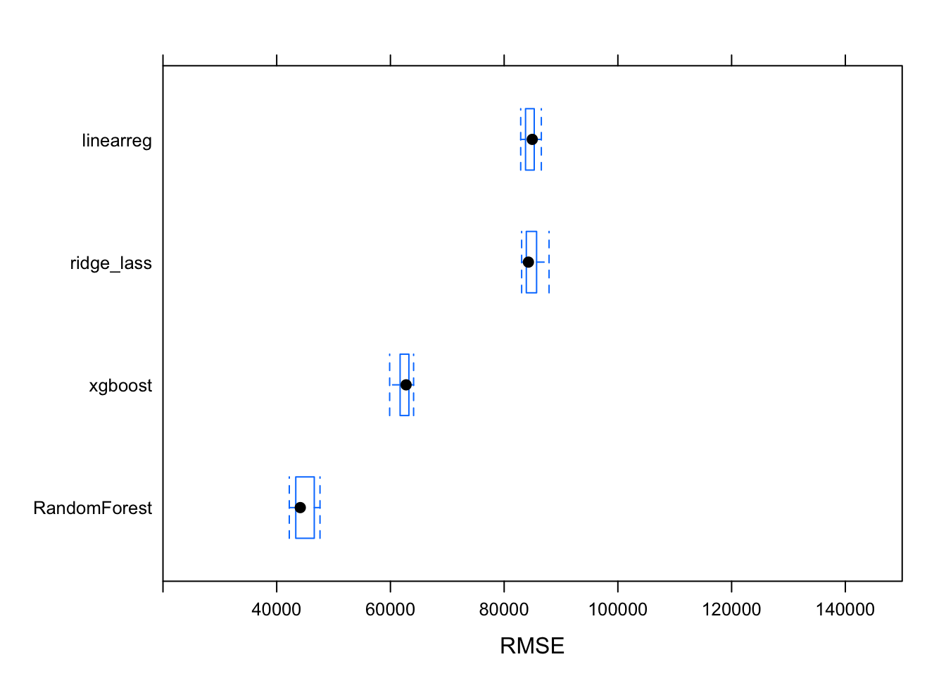
Great! We can see that the random forest model is doing significantly better than the rest, with a Root-Mean-Squared-Error of about $44,000. Let’s also check out this model’s performance on our test data.
rf_mod_fit = predict(rf_mod, test_data)

postResample(pred = rf_mod_fit, obs = test_data$price)
## RMSE Rsquared MAE
## 6.927496e+04 8.108359e-01 4.872507e+04The RMSE here is a lot higher than in our test data, and the Rsquared is certainly better than the linear regression (0.81 versus 0.6), it still leaves quite a bit to be desired. Let’s see if we can use some ensemble methods to improve performance.
Ensemble Models
First, we need to see if our models are good candidates for building an ensemble.
#Let's see how much correlation there is between model predictions - ideally, we want models that are fairly uncorrelated.
modelCor(results)
## RandomForest linearreg xgboost ridge_lass
## RandomForest 1.00000000 0.15752534 -0.09086445 0.53485131
## linearreg 0.15752534 1.00000000 0.61396724 -0.08224185
## xgboost -0.09086445 0.61396724 1.00000000 -0.34638214
## ridge_lass 0.53485131 -0.08224185 -0.34638214 1.00000000This looks promising! There is some moderate correlation between the outputs of the Ridge and Lasso model and the Random Forest model, but it’s not extremely high. This seems like a good candidate to build and test some ensemble models. Let’s use the caretList and caretEnsemble tools to buiild an ensemble model. We’re going to build a caretList object first, and then build three different ensemble types: a greedy ensemble, a glm ensemble and a random forest ensemble. A warning - these take significant time to build on a normal laptop. I’ll be loading previously built models for assessment below
#SEtting up the train control object
train_control = trainControl(method = "repeatedcv", number = 3, repeats = 3)

#Building the caret list
model_list <- caretList(
  price ~ ., data=train_data,
  trControl=train_control,
  metric="RMSE",
  methodList=c("lm", "ranger", "xgbTree", "glmnet"),
  tuneLength = 3
  )

#building a greedy ensemble
greedy_ensemble <- caretEnsemble(
  model_list,
  metric="RMSE"
  )

#glm ensemble
glm_ensemble <- caretStack(
  model_list,
  method="glm",
  metric="RMSE",
  trControl=trainControl(
    method="repeatedcv",
    number=3,
    repeats = 3
  )
)

#Random Forest meta-model
rf_ensemble <- caretStack(
  model_list,
  method="rf",
  metric="RMSE",
  trControl=trainControl(
    method="repeatedcv",
    number=3,
    repeats = 3
  )
)
model_list = readRDS("/Users/KeatonWilson/Documents/Projects/Tucson_Housing_Machine_Learning/output/model_list.rds")
greedy_ensemble = readRDS("/Users/KeatonWilson/Documents/Projects/Tucson_Housing_Machine_Learning/output/greedy_ensemble.rds")
glm_ensemble = readRDS("/Users/KeatonWilson/Documents/Projects/Tucson_Housing_Machine_Learning/output/glm_ensemble.rds")
rf_ensemble = readRDS("/Users/KeatonWilson/Documents/Projects/Tucson_Housing_Machine_Learning/output/rf_ensemble.rds")
greedy_fit = predict(greedy_ensemble, test_data)## Warning in predict.lm(modelFit, newdata): prediction from a rank-deficient
## fit may be misleadingglm_fit = predict(glm_ensemble, test_data)## Warning in predict.lm(modelFit, newdata): prediction from a rank-deficient
## fit may be misleadingrf_ens_fit = predict(rf_ensemble, test_data)## Warning in predict.lm(modelFit, newdata): prediction from a rank-deficient
## fit may be misleadingpostResample(pred = greedy_fit, obs = test_data$price)## RMSE Rsquared MAE
## 4.290985e+04 9.172482e-01 1.918544e+04postResample(pred = glm_fit, obs = test_data$price)## RMSE Rsquared MAE
## 4.290985e+04 9.172482e-01 1.918544e+04postResample(pred = rf_ens_fit, obs = test_data$price)## RMSE Rsquared MAE
## 4.521194e+04 9.078247e-01 2.047251e+04And there we have it - the best model on out-of-sample test data appears to be either the greedy model or the glm model, which have identical scores on test data, and not the more complex meta-models. We end up with an algorithm that predicts 91.7% of the variation in price, with an RMSE of $42,909 and an MAE of $19185. Not bad! We could go through with more complex tuning - but the computational time is getting a bit hairy. For now, this seems like a good predictive tool. Next steps will be implementing this model into a web-based tool that folks can use to assess the price of a house in Tucson!

