A note on munging…

This new data (much like the original data set) was extremely messy - it’s a tough task to work through multi-sheet Excel files with gaps, spaces and assorted errata. I’m going to skip over all of this - I don’t think there is anything particularly elegant about any of this code - it did the job, there are probably better and faster ways to do it, but it worked.

The new data and model

First, we’ll load the packages we need, and the new data frame that we’ll be working with (we’ll also do a bit of initial fiddling with tidyverse to get things ready):

library(tidyverse)
library(caret)


big_bean_monthly_ML = read_csv(file = "https://raw.githubusercontent.com/keatonwilson/beans/master/data/big_bean_monthly_ML.csv?token=AefUVL4PFtU0I0_M0akT_3smuKlSJTRLks5bq7NbwA%3D%3D")

big_bean_monthly_ML = big_bean_monthly_ML %>%
  mutate(month = factor(month), 
         class = factor(class)) %>%
  select(-date, -future_date, -future_month, -future_year) %>%
  filter(!is.na(future_avg_price)) %>%
  filter(class != "Lima") #Not a lot of Lima bean data - this will help clean things up. 

Now we’ll use caret’s built in partitioning and preProcessing to split the data into training and test sets and get it ready to do some model testing on. We’ll setup the control scheme for the train function later on. Here, we’ll do repeated cross-validation with 5 folds and 5 repeats within test data.

set.seed(45)
index = createDataPartition(big_bean_monthly_ML$future_avg_price, p = 0.80, list = FALSE)
ml_train = big_bean_monthly_ML[index,]
ml_test = big_bean_monthly_ML[-index,]

pp = preProcess(ml_train[,-9], method = c("center", "scale", "bagImpute", "YeoJohnson", "nzv"))
ml_pp_train = predict(pp, ml_train)
ml_pp_test = predict(pp, ml_test)

#Setting up the train control
fitcontrol = trainControl(method = "repeatedcv", number = 5, repeats = 5)

Now we can toss our training data on models. I tested a bunch of different models on this new data set (one of caret’s advantages): linear regression, artificial neural nets, keras, ridge and lasso regression, support vector machines, Extreme Gradient Boosted Trees, and the clear winner: Random Forest. Interesting, given this was the superior algorithm on the previous data as well. You’ll see summary statistics below. It’s also worth noting that there is some model tuning embedded in this train function -

(A warning - this takes a fair amount of time on my machine - probably around 45 minutes to an hour). We’re going to cheat and load the saved model object, but I’ll show the code for the model.

#Random Forest
rffit = train(future_avg_price ~ . , data = ml_pp_train,
              method = "ranger", trControl = fitcontrol, tuneLength = 15) 

Loading up the saved model object so I don’t have to chug through this every time I re-save the blog post. :)

rffit = readRDS(file = "/Users/KeatonWilson/Documents/Projects/beans2/models/rffit_full.rds") 

#A note here - I'm not pulling this from the github repo, even though it's on there, because I couldn't make readRDS play nice with pulling the file from a remote directory, so I'm just calling it directly from my machine. 

p_rffit = predict(rffit, ml_pp_test)
postResample(pred = p_rffit, obs = ml_pp_test$future_avg_price)

##      RMSE  Rsquared       MAE 
## 3.0370622 0.9083187 2.1029255

Great! We can see that this model generates a relatively high Rsquared and low RMSE on out of sample test data - it’s explaining around 91% of the variation in future average price, and our root-mean-squared error is $3.04/hundred weight of beans. It’s not quite as good as the last model - but it also incorporates a lot of variation that happened in the markets between 2010-2017.

New Insights

Let’s take a look at some of the plotting outputs from our model to see if we can refine our predictions a bit:

#binding predictions onto the test data frame
ml_pp_test$pred = predict(rffit, ml_pp_test)

#Plotting predictions versus actual future prices
ggplot(ml_pp_test, aes(x = future_avg_price, y = pred, color = class)) +
  geom_point(size = 2, alpha = 0.6) +
  theme_classic() +
  geom_abline(intercept = 0, slope = 1)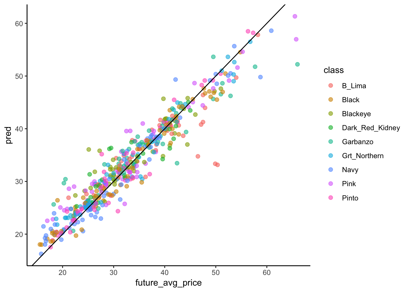

We saw this plot before. If our model was 100% accurate, every dot would be on the 1:1 line. It’s not, but it’s doing a good job overall. There are a couple of questions that come out of this figure.

First, we can ask whether the model consistently under- or over-predicts price for certain classes of beans, which might help us to make better purchasing decisions, and second, it looks like the model typically over-predicts prices of low value and under-predicts prices of high value. We can test both of these things quantitatively.

ggplot(ml_pp_test, aes(x = future_avg_price, y = pred, color = class)) +
  geom_point(size = 2, alpha = 0.6) +
  theme_classic() +
  geom_abline(intercept = 0, slope = 1) +
  facet_wrap(~ class)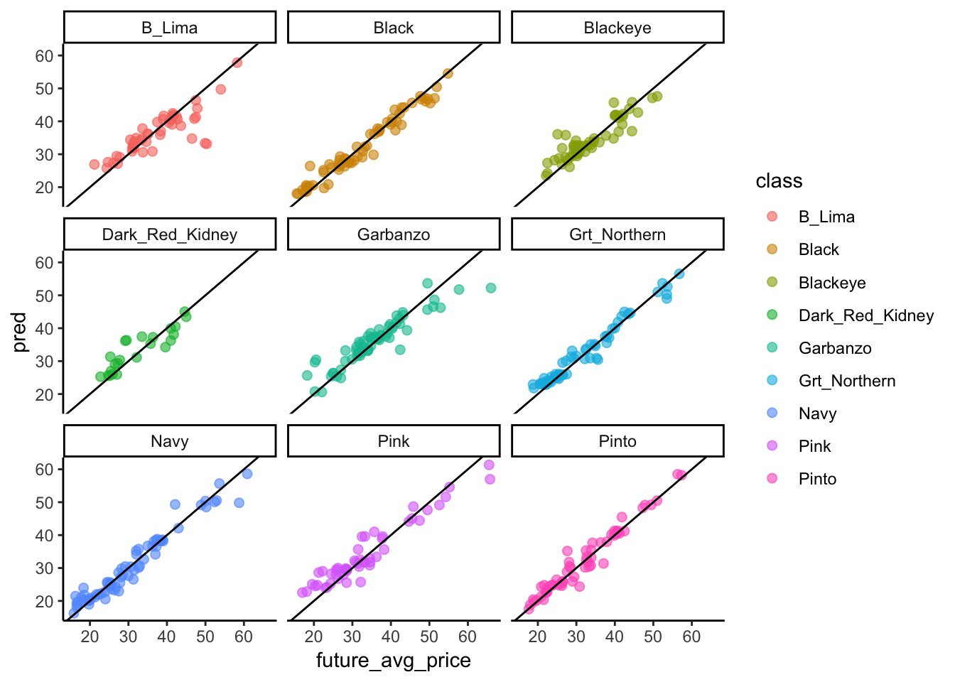

ml_pp_test %>%
  group_by(class) %>%
  dplyr::summarize(mean_residual = mean(pred - future_avg_price)) %>%
  arrange(desc(mean_residual))

## # A tibble: 9 x 2
##   class           mean_residual
##   <fct>                   <dbl>
## 1 Pink                  0.821  
## 2 Dark_Red_Kidney       0.755  
## 3 Blackeye              0.696  
## 4 Grt_Northern          0.485  
## 5 Garbanzo              0.416  
## 6 Pinto                 0.372  
## 7 Navy                  0.00654
## 8 Black                -0.193  
## 9 B_Lima               -1.03

So, we can tell that the model doesn’t predict equally well for all classes - and the summar table breaks this down. The mean_residual column shows the average amount each class is off by. For example, the model consistently over-predicts the price of pinks and under-predicts the price of Baby Limas. Good information to have if one were to use this model to make purchasing decisions!

Let’s look at differences between high prices and low prices!

q = quantile(ml_pp_test$future_avg_price)
ml_pp_test %>%
  mutate(quantile = cut(future_avg_price, q, labels = c(1,2,3,4))) %>%
  group_by(quantile) %>%
  dplyr::summarize(mean_residual = mean(pred - future_avg_price)) %>%
  filter(!is.na(quantile))

## # A tibble: 4 x 2
##   quantile mean_residual
##   <fct>            <dbl>
## 1 1                1.78 
## 2 2                0.854
## 3 3               -0.116
## 4 4               -1.60

ggplot(ml_pp_test, aes(x = future_avg_price, y = pred, color = class)) +
  geom_point(size = 2, alpha = 0.6) +
  theme_classic() +
  geom_abline(intercept = 0, slope = 1) +
  geom_smooth(method = "lm", linetype = 2, aes(group = 1), color = "black")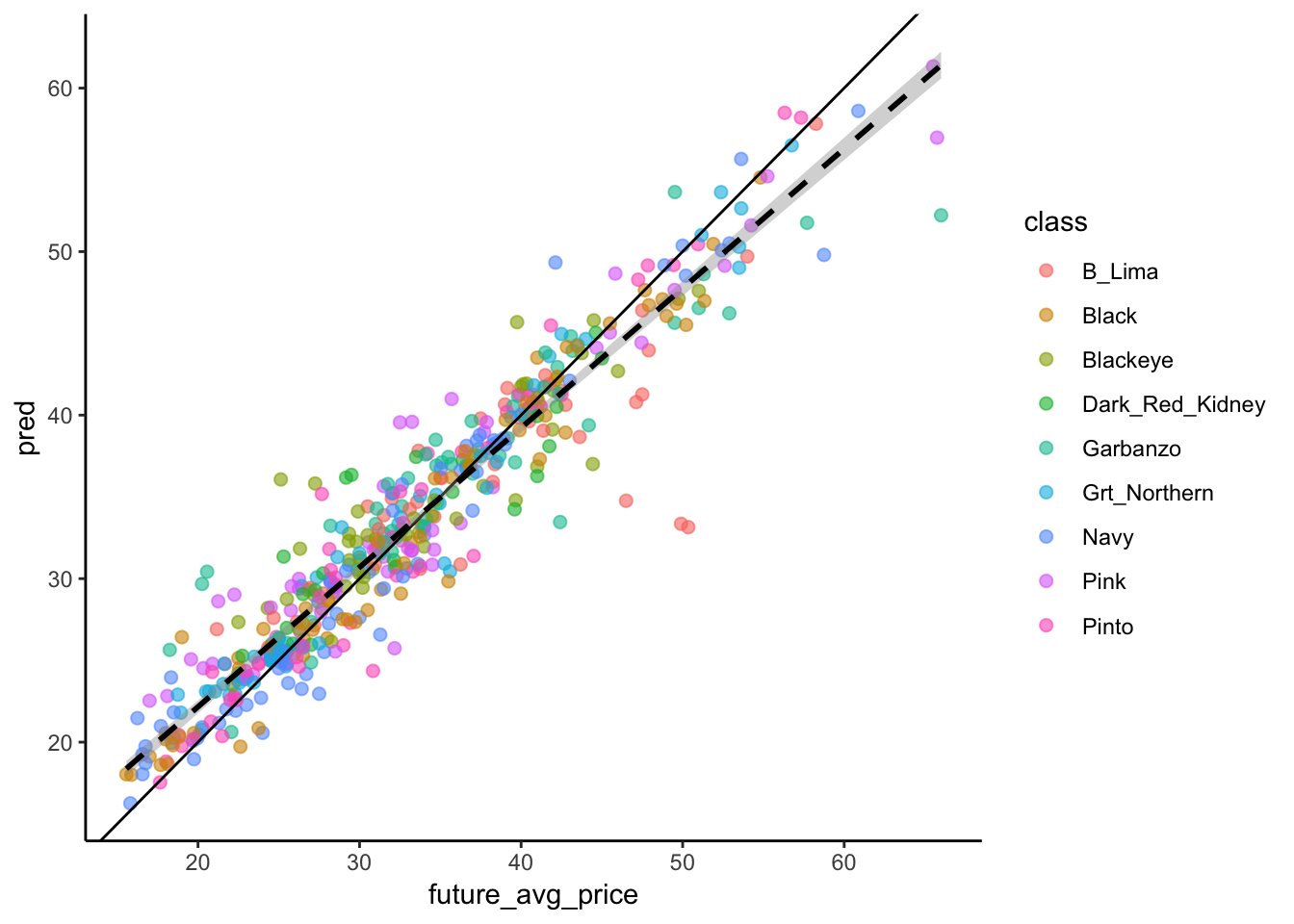

We can see that the model in fact over-predicts beans at low price and overpredicts beans of high price by the table and figure above. The table shows the mean difference between prediction and actual price across each of the quantiles of the data (the bit at the low end, bits in the two middle chunks, and bits at the high end), and a linear model of data shows that it isn’t parallel with the 1:1 line. Again, good information to have if you were trying to make informed bean-purchasing decisions.

Conclusions

So, in summary, we now have a very nice complete data set of bean prices, production and imports that leads to a strong predictive model of price 6 months in the future across all varietals. Though it’s predictive power is slightly lower than the previous model, it incorporates a wider swath of time and more recent variability in the market. We’ve also developed a couple of analytical tools to examine the model output that would allow us to make more informed decisions about purchasing when making decisions among varietals that are priced higher or lower.

Cheers!